Deep learning via CNN for identification of blue core phenomenon in helicon plasma discharge

Abstract

Based on deep learning image recognition techniques, a Convolutional Neural Network (CNN) model for discharge modes recognition of helicon plasma was trained. The accuracy of the model was evaluated using functions such as F1-score and confusion matrix. The final recognition accuracy was more than 98.18% after 30 iterations. Interpretable analysis was done using methods such as Gradient-weighted Class Activation Mapping (Grad-CAM) to verify the model’s robustness as well as repeatability. The model identification results were compared with Langmuir probe diagnostic results. It was found a good fit between the model and the probe results, corroborating the correctness of the model. The present model can well identify the critical power of entering W mode in the discharge process of helicon plasma. As the discharge database expands, it has great potential for recognizing the higher-order discharge modes based on the deep learning.

Keywords: helicon plasma, mode transition, deep learning, Convolutional Neural Network (CNN),image recognition

I.INTRODUCTION

Helicon plasma has great application prospects in the fields of astronautics propulsion, magnetic confinement fusion, and material surface treatment due to its high plasma density of up to 1020 m-3 under the conditions of low gas pressure (0.01-10 Pa) and low magnetic field (<1000 G). Helicon plasma is generated by the energy deposition of radio frequency (RF) power source through antenna coupling with an external magnetic field. Mode transition is one of the most interesting features of helicon plasma. Three different discharge modes, capacitive (E), inductive (H), and helicon (W) modes can be identified among the helicon plasma discharge process. After the plasma enters the W mode discharge, the discharge center shows a bright blue color, a phenomenon known as blue-core, which is another important feature of helicon plasma discharge. Zhang and Cui et al.4, 5 found that blue-core generally appeared in helicon modes with strong magnetic field and high plasma density, accompanied by an exponential increase in the ion line strengths, the electron density and its temperature, ion density and its temperature, and line emission intensities showed radial distributions with central peaks in the blue-core mode. Wang et al. explored the effect of inhomogeneous magnetic field as well as neutral gas pressure on the blue-core phenomenon in helicon plasma. Lu et al. excited the blue-core phenomenon using a magnetic field of 2000 G and a Nagoya III antenna to explore the effect of a magnetic field configuration with a zero magnetic point on the plasma parameters. Xia et al. designed dual magnets, placed at both ends of the antenna, and excited blue-core phenomena at lower power(~200 W).

The identification approach for the mode transition in the helicon plasma is mainly based on the RF-compensated Langmuir probes to eliminate interference from RF signals10, 11. The high temperature of helicon plasma can damage the probe, making it more difficult to measure plasma parameters at high power. Another commonly used diagnostic method to identify the mode transition in helicon plasma is non-invasive optical emission spectroscopy (OES)12. However, it may be invalid for the spatial-resolved diagnosis due to the spectra recorded from a large bulk of
plasma13. The integrated capacitively coupled detector (ICCD) is also occasionally used to diagnose the state of helicon plasma discharge14. However, it is often a qualitative description and comparison. It can be seen that the experimental approaches are often limited by the experimental conditions, the measurable range, the accuracy of the obtained data, and some experimental results cannot be quantitatively analyzed.

With the development of artificial intelligence, there are more and more researches on analyzing physical phenomena of plasma discharge through machine learning. Deep learning is a branch of machine learning based on Deep Neural Networks (DNNs), meaning neural networks with at the very least 3 or 4 layers. Wang et al.15 proposed a DNN with multiple hidden layers as an example to replace the fluid model to accurately describe the essential discharge features of CO2 pulsed discharge under Martian conditions. They found the constructed DNN can achieve a satisfied prediction performance. Compared to the fluid model, the DNN takes only a few seconds to predict the discharge characteristics and profiles of the electric field, particle density, and the spatial–temporal distribution of the given products in CO2 plasmas. Kates-Harbeck et al.16 present a deep learning-based method for predicting outages in magnetically confined Tokamak reactors,which opens up the possibility of moving from passive outage prediction to active reactor control and optimization. Cheng et al.17 compared the accuracy and speed of traditional machine learning and deep learning in predicting energy deposition in helicon plasma, and found that DNNs showed better stability in response to changing conditions compared to traditional algorithms.

Convolutional Neural Network (CNN) is one of the most popular neural network architectures18. The first report of CNN came in 1989 when Lecun et al. used a backpropagation network to recognize handwritten digits19. CNNs, designed to process data in the form of multiple arrays, have been successfully applied for detection, segmentation and recognition of objects and regions in images. Image recognition techniques have been successfully applied in a number of fields20. James et al.21, 22 used image recognition techniques to predict the two-dimension (2D) appearance of a silicon sample surface directly during ablation by a single-pulse femtosecond laser. Matos et al.23 used a DNN to produce a full, pixel-by-pixel reconstruction of the plasma profile. The network could provide accurate reconstructions with an average pixel error as low as 2%. Kim et al.24 used machine learning technique to classify discharge states of Tokamak based on raw edge reflectometer data in real-time. The trained CNN models achieved a classification accuracy of up to 99%. However, to the best of our knowledge, there has been no report on the application of CNNs for the identification of mode transition and blue core phenomenon in helicon plasma discharge.

In this paper, deep learning based on CNNs will be used to classify the images captured by camera in order to find the critical point where the blue core phenomenon occurs in helicon plasma discharge process. This paper is structured as follows: Section I provides a brief history of helicon plasma discharge and deep learning. In Section II, we will describe the helicon plasma discharge system and CNNs model used in the paper. Section III discusses the model performance. Finally, Section IV proposes a conclusion on this work.

II. EXPERIMENTAL SYSTEM AND SIMULATION MODEL

A. Helicon plasma apparatus

The experimental setup is shown in Fig. 1, where the plasma was generated in a cylindrical quartz tube of 3 cm in diameter and 45 cm in length, with a water-cooled RF antenna mounted outside the quartz tube. One end of the discharge tube was sealed by a stainless steel plate, and the other end was connected to a stainless steel expansion chamber with a diameter of 10 cm and a length of 14 cm. The discharge tube was surrounded by a water-cooled Nagoya Ⅲ antenna and connected to an RF generator (13.56 MHz, 0-2000 W, RSG-2000 Rishiger Electronic Technology Inc.). In order to keep the reflected power below 1% of the input power, an auto-matching L-shaped network was placed between the Nagoya Ⅲ antenna and the RF generator. The discharge tube was located in an inhomogeneous field induced by a collection of four annular neodymium-iron-boron (NdFeB) permanent magnets with an inner diameter of 4.8 cm, an outer diameter of 9 cm, and a thickness of 1 cm, as well as four insulating plates of the same size. The vacuum inside the chamber consists of a turbomolecular and mechanical pump, and argon gas was continuously supplied to the chamber from the upper end of the discharge tube.

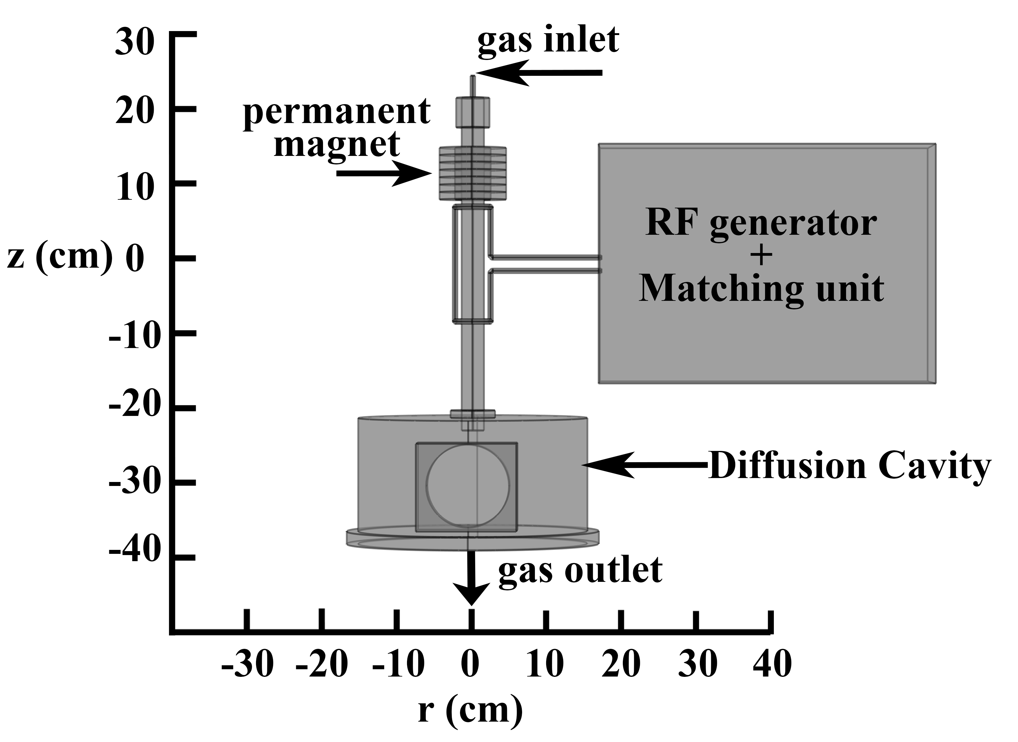
This experiment was conducted at the power scale of 0-1010W. The working gas pressure was fixed at 0.36 Pa. The magnetic field strength was lower than 300 G. NikonD90 camera was placed in front of the discharge equipment at 0.5 m, horizontally aligned with the discharge tube, the focal length was selected as 105 mm. The aperture, shutter speed and International Organization for Standardization (ISO) of camera were set to f/4, 1/20s, and 3200, respectively.

B. Convolutional Neural Network model

Because of the limited ability to capture images of helicon plasma discharges in this experiment, the data obtained was trained through transfer learning, which is used to improve a learner in a domain by transferring information from related domains25. The ResNet-18 model was used to initialize the training model, and on the basis of which transfer learning was carried out in order to obtain a model that was suitable for this research. ResNet-18 is a deep residual network proposed by Microsoft Research to solve the problem of gradient vanishing and gradient explosion during deep neural network training. It is a smaller model in the ResNet family with 18 layers of depth. The input data was first passed through a convolutional layer, a pooling layer and a ReLU (Rectified Linear Unit) layer, then through four 3*3 convolutional layers, the output to an average pooling layer, and most of all a linear layer was used to transform the output.

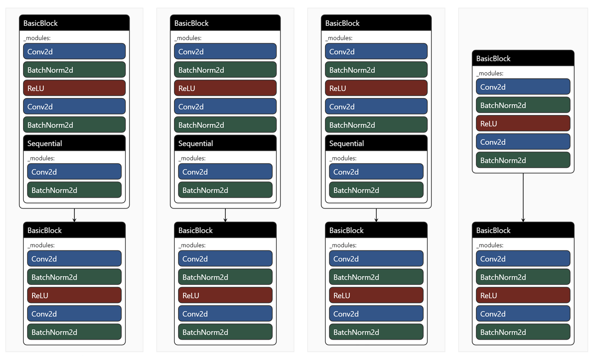
Figure 2 shows the structure of the BasicBlock module in a ResNet network architecture. The BasicBlock is the basic unit of residual block in ResNet, which consists of two convolutional layers and a group of residual connection, i.e., Conv2d, BatchNorm2d, and ReLU. Conv2d is a 2D convolutional layer used to extract spatial features from the input feature maps. There are two Conv2d layers in a BasicBlock, each of which performs convolutional operations using a 3x3 convolutional kernel. BatchNorm2d is a batch normalization layer used to normalize the output after convolution. This speeds up the convergence of the network and stabilizes the training process. ReLU is the activation function layer that passes the output values through the nonlinear function ReLU to increase the nonlinear capability of the network. A Sequential module will be included in some BasicBlocks to adjust the shape of the inputs to match the dimensions of the subsequent operations (e.g., when the number of channels in the inputs and outputs are different or when the resolution of the feature map changes). This Sequential module will usually contain a convolutional layer and a batch normalization layer. This method is the residual connections, which serve to directly skip from the input to the output so that the gradient of the network can be propagated more directly. This effectively mitigates the problem of vanishing gradients that occurs in deep neural networks. The BasicBlock in the first and second columns of the Fig. 2 both contain Sequential modules, which means that in these residual blocks, the number of channels in the input needs to be changed (e.g., increased from fewer to more channels.). The Sequential module contains a convolutional layer and a batch normalization layer to achieve this. The two BasicBlocks in the third and fourth columns do not have a Sequential module, indicating that the number of channels in the input is the same as the number of channels in the output. The residual connection can be used to directly add the input and the convolved output. The design of these BasicBlock modules allows the network to be trained more efficiently while increasing its depth. With the introduction of residual connections, the network can better convey gradient information and reduce training difficulties, thus improving the performance of deep learning models.

C. Methods of outcome evaluation and interpretable analyses

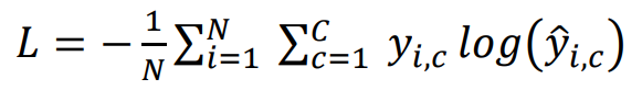
The cross-entropy loss function was used to prevent model overfitting26 and evaluate the performance of trained model27 by calculating the loss value between true label and predicted label. The cross-entropy loss function usually indicates how well the model fits the training data with the current parameters. The loss value calculated by the loss function can be used as the gradient information in the back-propagation algorithm to update the model parameters using optimization algorithms such as gradient descent, enabling the model to be continuously optimized to better fit the training data and improve model performance. In the model training process, the cross-entropy loss function adjusts the parameters of the model by minimizing the loss value, making the model’s prediction results closer to the real label. When the model’s predictions are exactly in line with the real label, the cross-entropy loss reaches a minimum of 0. Overall, the loss function serves to provide feedback optimization signals, guide the adjustment of model parameters, and evaluate the model performance. It is a key component in the model training and optimization process. The cross-entropy loss function (L) used in this experiment is:

where 𝑁 denotes the number of samples, 𝐶 denotes the number of categories, and 𝑦𝑖,𝑐 are the true labels of sample 𝑖.

Accuracy, Precision and Recall are metrics used to evaluate machine learning algorithms for understanding the performance of classification models28 . Accuracy is the ratio of total correct samples to the total samples. Accuracy can be calculated as:

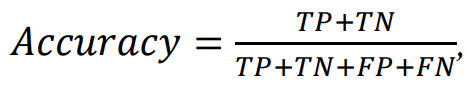
where TP (True Positives) denotes the model correctly predicted a positive outcome, i.e., a case where the true value of the data is a positive case and the predicted value is also a positive case. TN (True Negatives) is a negative case that was correctly predicted as a negative case. FP (False Positive) is a positive case that was incorrectly predicted, i.e., a case where the true value of this data is a negative case, but was incorrectly predicted as a positive case. FN (False Negatives) is a positive case that was incorrectly predicted as a negative case.

Precision is a measure of how accurate a model’s positive predictions are. It is defined as the ratio of correctly classified positive samples to a total number of classified positive samples (either correctly or incorrectly). Precision can be calculated as:

Recall measures the ability of the model to correctly identify all true positive examples, i.e., the probability that the identification is true in a positive sample. A high Recall means that the model is better able to cover all true positive examples and avoid missing important samples. Recall can be calculated as:

A good model needs to strike the right balance between Precision and Recall29 . F1-score (F1) takes into account the Precision and Recall of the classification model, and provides a more comprehensive assessment of the model’s performance between positive and negative categories30 . For imbalanced datasets, the use of Recall alone may cause bias when evaluating model performance, while F1-score can more accurately evaluate the overall model performance. F1-score can be calculated as:

The confusion matrix was used to visualize the classification of the model on different categories and then calculate various evaluation metrics31 .The interpretability of the model was analyzed using the Gradient-weighted Class Activation Mapping (Grad-CAM) method32, which will be introduced in the next part.

III. RESULTS AND DISCUSSION

A. Image acquisition results

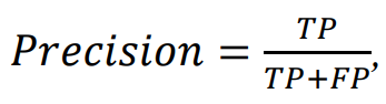
A total of 828 images were captured for this experiment, in which 218 images were labeled as H mode and 610 images were labeled as W mode. These images were divided into a training set and a validation set. In addition to interesting region, images taken directly from discharge experiment often include background shielding grid around the discharge tube used to minimize RF interference. It is necessary to crop the image to retain the key region of interest. Two typical cropped images are shown in Fig. 3. Figure 3(a) and 3(b) are labeled as discharge image in H mode and W mode, respectively. The cropped image is no longer affected by the RF shielding grid. The CNN model can better focus on the discharge tube itself, increasing its interpretability and accuracy. Normally, cropped images need to be rotated and normalized before being put into model for training20. The image pre-processing can increase the randomness of the images, improve feature extraction by eliminating irrelevant information from the image and enhance the detectability of relevant information.

B. Accuracy assessment

This experiment only adopts the architecture of ResNet-18 model, but does not load its pre-trained weight parameters. This experiment was designed with 30 epochs of iterations, taking into account the cross-entropy loss function, Recall and other metrics to fully assess the accuracy and generalization ability of the model. Figure 4 shows the evaluation results of several functions in detail. As can be seen by pulling the log, the model quickly finds the optimal gradient. In the first 10 batch the cross-entropy loss function has already converged to less than 0.5, as shown in Fig. 4(a). After the third epoch of training, the cross-entropy loss function has dropped to a low order of magnitude, as shown in Fig. 4(b), and eventually keeps approaching the 0. The accuracy is more than 90% and tends to grow steadily, as shown in Fig. 4(c). These are attributed to the good performance of the ResNet-18 architecture in finding the optimal gradient. Figure 4(d) illustrates several other assessment indicators, Accuracy, Precision, Recall and F1-score, tend to stabilize after the sixth epoch and keep approaching 98%. After 30 epochs of iterative training, the optimal model is obtained with an accuracy of 98.18%.

The confusion matrix can be used to visualize the classification of the model on different categories and then calculate various evaluation metrics31. Precision-Recall (PR) curve shows the relationship between Precision and Recall of the model at different thresholds33 . The PR curve mainly evaluates the performance of a model when facing different datasets. It focuses on the TP and is sensitive to the sample proportion, so it can show the effect of the classifier with the change of sample proportion. The ability of a classifier to classify an imbalanced dataset can be measured based on the results exhibited by the PR curve34, which can be used for model improvement and optimization. In this work, W mode has far more images than H mode, so the PR curve can give a clearer picture of the model’s performance on the minority class. The Receiver Operator Characteristic (ROC) curve shows the relationship between True Positive Rate (TPR, also known as Recall) and False Positive Rate (FPR) of the model at different thresholds35 . It is mainly used when the distribution of samples in the test datasets is relatively balanced. The ROC curve keeps basically unchanged when the distribution of positive and negative samples in the test datasets changes. The stability of ROC curve in the face of imbalanced datasets suggests that it can present an overly optimistic performance of a model itself. However, this insensitive nature makes it difficult to see how a model predicts when faced with a sample change in the imbalanced datasets. In other words, the PR curve is more informative than the ROC curve when evaluating binary classifiers on imbalanced datasets28 .

Figure 5(a) and 5(b) show the PR curve and ROC curve of the model, respectively. The PR curve of this model is concentrated in the upper right corner of the graph and the ROC curve is concentrated in the upper left corner of the graph, which indicates that this model has excellent accuracy. The Area Under the Curve (AUC) measures the overall performance of the binary classification model. It will always lies between 0 and 1 due to the Precision and Recall in PR curve or TPR and FPR in ROC curve range between 0 to 1. A greater value of AUC denotes better model performance. It has been calculated that the area under the PR curve (PR-AUC) is greater than 0.98 for both classifications, and the area under ROC curve (ROC-AUC) is greater than 0.99. It represents the probability with which our model can distinguish between the two discharge modes.

Figure 5(c) shows the confusion matrix for the binary classification of H mode as positive class and W mode as negative class. A total number of 165 images have been contained in the test dataset, as shown in the sum of the numbers in all the boxes. It can be seen from the first column that the total images in the H mode are 45. Similarly, the second column gives us the numbers of images in the W mode are 122. The correct classifications are the diagonal elements of the matrix, e.g., 42 for the H mode and 120 for the W mode. It means a total of 162 images were correctly predicted out of the total 165 images. Thus, the overall accuracy is 98.18%. Out of the 165 images in the test dataset, only 3 images were classified incorrectly, 1 image of which was originally in H mode discharge, as shown in Fig. 5(d), which was taken at 180 W and was classified as W mode. In addition, the next 2 images, which were originally in W mode discharge, were recognized as H mode. The quantitative evaluation metrics, Accuracy, Precision, Recall and F1-score, can be calculated using these four different numbers from this binary class confusion matrix, as illustrated in the Table 1. The Precision, Recall and F1-scores are 97.67%, 95.45%, and 96.37% for H mode as positive class, respectively. When W mode is used as the positive class, the corresponding metrics are 99.17%, 98.36%, and 98.99%, respectively. These metrics show that the model performs well for both H mode and W mode, and that the model performs better when it recognizes W mode.

C. Interpretability analysis

Interpretability analysis reveals areas of discharge that the network model focuses more on in distinguishing mode transitions, which can be used as a guide for experimental diagnosis. Selvaraju et al.32 have proposed a technique, Gradient-weighted Class Activation Mapping (Grad-CAM), to provide a “visual interpretation” of the decisions of a large number of CNN based models, where a linear neuron importance weights combination of forward activation maps is followed by a ReLU layer to compute the convolutional layer (𝐿 𝑐 ) of a given image through the saliency map:

where 𝑤𝑘 𝑐 is the neuron importance weights of feature map 𝑘, 𝐴 𝑘 is the feature activation map 𝑘. In this algorithm, an image and a category of interest (e.g., image of W mode discharge in this work) as input, which is propagated forward through the CNN part of the model to obtain a gradient score y for the category. Setting the score for desired category to 1 and the others to 0. This signal is then global-average-pooled and combined with a ReLU to obtain the coarse Grad-CAM heat map that highlights important regions of the predicted concepts in the image32 . Grad-CAM++ can be understood as an upgraded version of Grad-CAM, which adds an extra weight to the elements of the gradient map relative to Grad-CAM, making the localization more accurate and suitable for multi-target detection36. Therefore Grad-CAM++ was preferred at the beginning of this experiment to analyze the interpretability of the images to be recognized. It can be seen from the heat map showed in Fig. 6(a), similar to the direct observation of helicon plasma discharge images by the human eye, the computer also focus on the central region of the discharge images. According to the radial plasma density results reported in our previous work6 , the discharge in the central region will be stronger and accompanied by the appearance of a blue core. The present model also demonstrates the discharge state of the helicon plasma through this phenomenon.

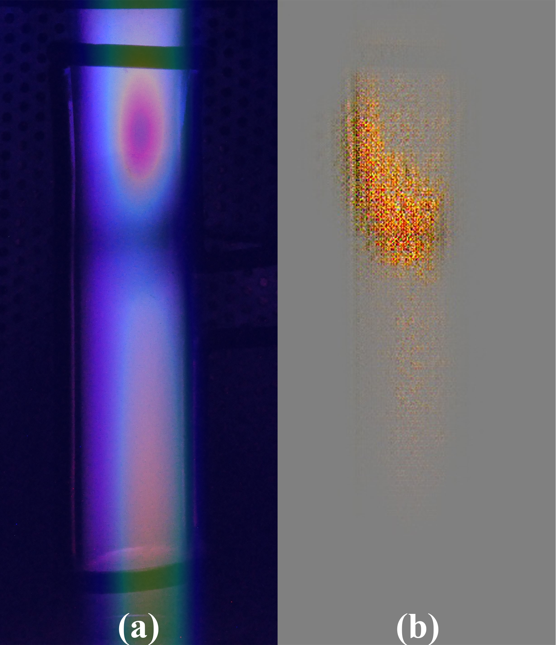
However, the Grad-CAM family lacks the ability to demonstrate fine-grained significance like the pixel-space gradient visualization method. The result of Guided Backpropagation33 was combined to Grad-CAM heat map by means of dot-multiplication to realize a high-resolution class-discriminative visualization. This technology is also referred to as Guided Grad-CAM32, the heat map drawn by this technique is shown in Fig. 6(b). It shows that the region where the computer quantitatively identifies the W mode is shown at a finer granularity by fitting the region of the original image. It can provide a guiding direction for the future discharge diagnostics of helicon plasma such as the placement of the OES fiber.

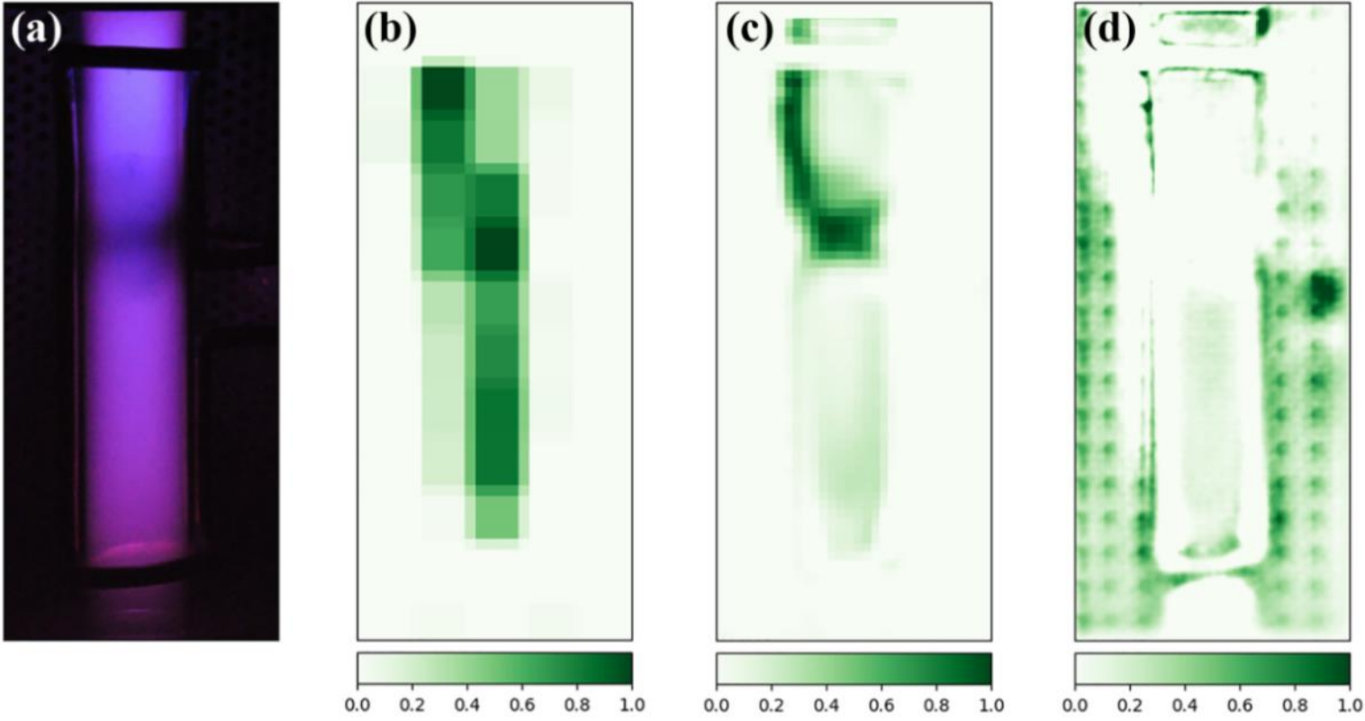
To further verify the effect of confusion on the stability of the recognition system, captum, an model interpretability and understanding library37 , has been used to design sliders of different sizes to mask the recognized image for the aim of testing which areas masked have the greatest effect on the system’s ability to recognize the discharge state. Three different sizes of sliders, large, medium and small, were designed. The results of the experiment are shown in Fig. 7. The effect of the large slider masking on the system is most consistent with the results observed by the human eye, with the area of effect centered on the upper part of the discharge tube, the main area where the blue core is generated, as shown in the Fig. 7(b). By observing Fig. 7(c), the most affected place is located at the end of the blue core, so the exploration of the axial length of the blue core becomes a feasible direction. And Fig. 7(d) mainly demonstrates the effect of pixel points near the antenna on the recognition of the discharged pictures. This set of experiments not only confirms the robustness of the model but also provides a reasonable direction for future research.

D. Comparison of training results with Langmuir probe results

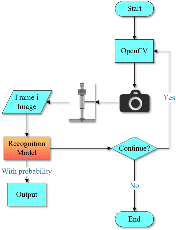
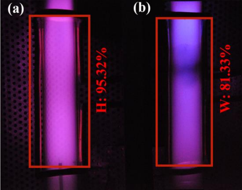
After completing training the model, a recognition system has been built, which can identify the W mode discharge with blue core phenomena in helicon plasma in real time. The specific flowchart is shown in Fig. 8. This system consists of a camera that acquires discharge images of helicon plasma in real time with an acquisition frame rate of 25 fps. The system calls the camera to capture real-time images through the OpenCV plug-in. The ith frame is passed into the system for pre-processing such as resizing, normalization and denoising and then into the recognition model. The model prints the judgement result on the ith frame and outputs it on the screen in real time. Two typical Real-time screen output from the identification system are shown in Fig. 9, which contains the identified discharge modes as well as the probabilities, respectively. It can be seen that the discharge mode is H mode with the probability of 95.32% in Fig. 9(a) and W mode with the probability of 81.33% in Fig. 9(b).

The results obtained by the recognition model were compared with the ones given by Langmuir probe technique at the same RF power in our previous work38, as shown in Fig. 10, where the black squares and solid line is the plasma density curve following the applied powers and the black spheres and solid line is the mode curve recognized by the picture identification system. At the power of around 200 W, the density of helicon plasma discharge detected by the probe undergoes a sharp increase, i.e., it jumps from the H mode to the W mode. At the same time, a blue-core phenomenon occurs monitored by the real-time identification system at ~200 W, which confirms the good stability and repeatability of the identification system based on deep learning model. The recognition system can identify the discharge mode in real time, faster than the experimental prober diagnostic methods. At the same time, it is a non-invasive method. It can determine the discharge mode of helicon plasma without disturbance. It is accurate enough to be used to determine the W mode if the helicon plasma discharge with blue core phenomenon.

IV. CONCLUSION

In this paper, a novel deep learning method for identification the mode transition in helicon plasma discharge is presented. The method is based on convolutional neural network and residual neural network with 18 layers depth. The plasma discharge images are simply cropped and fed into the network. The accuracy of the constructed deep learning model can up to 98.18%. Furthermore, the Grad-CAM algorithm is used to give a heat map of the computer-recognized discharge image, which confirms the reasonableness of the model and also gives the direction for experimental diagnosis. Based on the deep learning model, the discharge modes with the probabilities of helicon plasma are recognized by the real-time identification system, which has good stability and repeatability compared with the experimental results. The real-time identification system can be improved by enriching the experimental image data for mode transition recognition of helicon plasma under complex conditions in the future.